Protocols

title: “Coral Tissue separation & Chl/Zooxanthellae Counts Protocol” output: html_document —

Part 1: Coral Tissue separation

Start with tissue removal and prepping samples for zoox counts and pigments, samples can be frozen in their Eppendorf tubes until we’re ready to do the pigment analysis and zoox counts

1. Primary processing

  1. Filter 1 liter of fresh seawater
  2. Clean the coral fragment with toothbrush, rinse it in SW
  3. Place coral fragment in ziplock bag and seal it around the water pick. Hold fragment near top of bag from the outside to allow slurry to drop into bottom of bag while allowing for good visualization of fragment.
  4. Remove the tissue from entire coral fragment with water-pick using filtered seawater (0.7µm-filtered) until skeleton is white (adjust pressure to 10, don’t want to blow a hole in the bag, but strong enough to remove tissue quickly) ** use water conservatively. Try to remove all tissue with two rounds of 45 mL FSW, but can use more if needed.
  5. Rinse fragment when white one final time
  6. Pour the tissue slurry (blastate) into labeled 50 ml Falcon tube
  7. Rinse walls of bag ONCE with additional 5 mL of FSW and add to Falcon tube
  8. Record final blastate volume and adjust samples to equal volumes
  9. Homogenize blastate for 30 seconds using a vortex genie, use homogenizer to break up chunks if necessary
  10. Centrifuge blastate for 15 minutes at 4,500 rcf
  11. Label the cleaned skeleton and save for surface area via aluminum foil

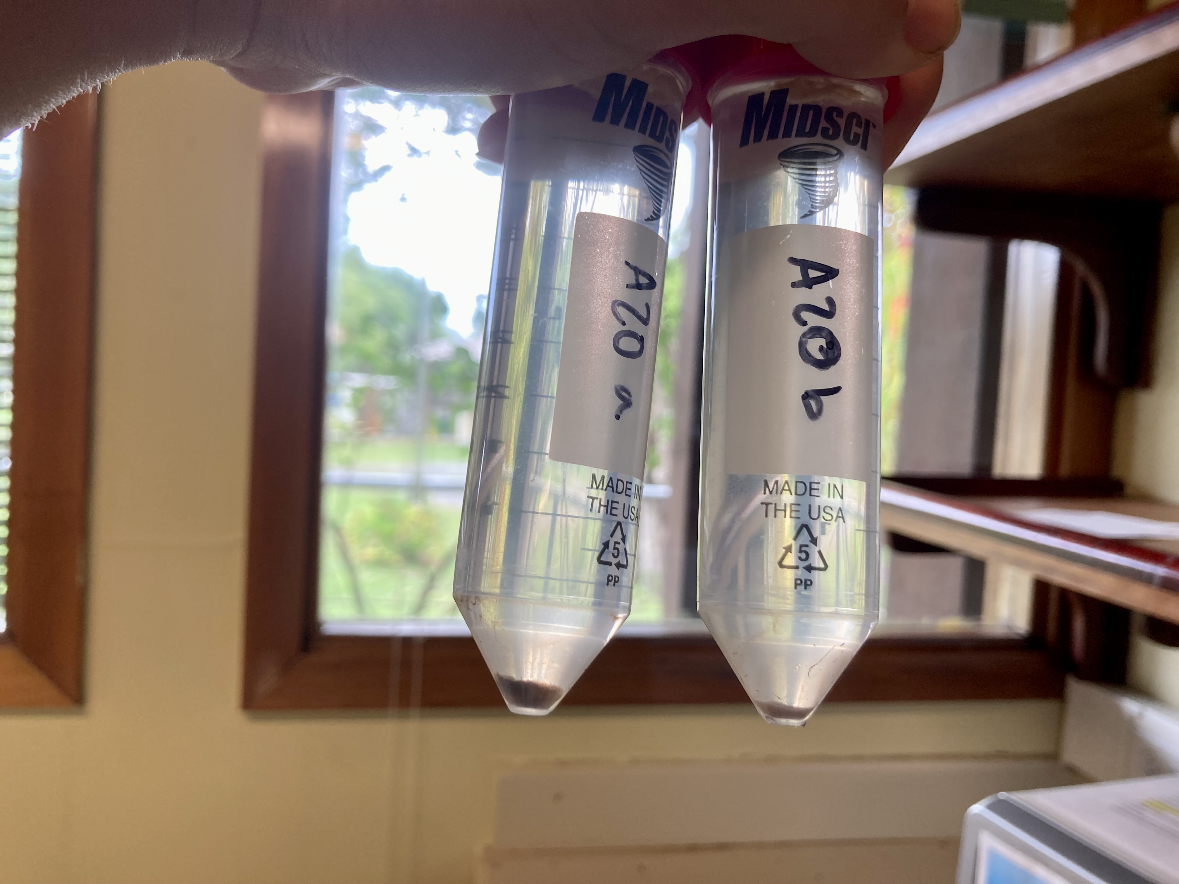
caption: Animal portion floating at the top, algae pellet at bottom.

2. Separation of tissue types – Animal Tissue

  1. Pour the supernatant off from first spin (this is the top layer in the tube and is the ANIMAL fraction). This will leave behind a green/tan pellet—this is the “algae fraction” with some remaining animal tissue (this is what we want for chl a and counts)
  2. Add 0.75 ml FSW to algal pellet (epp. tube can only be filled to 1.1 mL or it will overflow while homogenizing)
  3. Vortex until pellet breaks apart (around 30-60 seconds)
  4. Mix resuspended pellet with pipette and transfer to Eppendorf tube
  5. Homogenize the algal fraction on high for 30 sec. 
  6. Rinse 50 mL falcon with FSW squirt bottle and fill Eppendorf tube to 1.5 mL line with pipette, vortex 10 seconds.

#(need images homogenizing algal pellet)

3. Washing Zoox

This cleans off bits of cell debris and nematocsysts that can be confused for zoox cells during counts

  1. Centrifuge the resuspended pellet for 5 minutes at 4,500 rfc
  2. Pour the algal fraction supernatant into the waste beaker
  3. Add 0.5 mL FSW to the algal pellet for first round (to combine epp tubes into one per fragment), 0.75 mL for second round of cleaning.
  4. Vortex until pellet breaks apart (around 30-60 seconds)
  5. Homogenize (15 sec) and combine with 2nd Eppendorf tube from fragment/sample. Fill tube to 1.5 mL and vortex (10 seconds)
  6. Centrifuge at 7,000 rfc for 3 min
  7. Repeat steps 2-6 two more times, use 0.75 mL FSW in step 3.

4. Prepping the zoox for chl a and for zoox counts

  1. Resuspend the cleaned zoox pellet in 1 mL of FSW (use vortex, homogenizer, and pipette to mix the sample well before taking the aliquot) , add 0.25 ml of seawater after homogenizing and vortex.

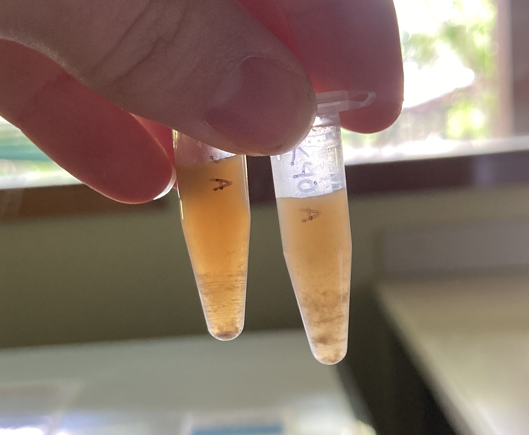
caption: Homogenized algal fractions, ready for aliquot.

  1. Transfer a 100 uL aliquot to a labeled eppendorf tube
  1. This is for raw hemocytometer counts
  1. Transfer 2 separate aliquots of 0.25 mL to 2 epi tubes for PIGMENTS (2 pigment replicates per coral sample) and freeze
  2. Freeze the remaining 0.5 mL in epi tube for ARCHIVE ( this is our backup)

** You now should have 4 eppendorf tubes to be frozen (1 for zoox counts, 2 for pigments, 1 archive/extra)

Part 2: Chl/Zooxanthellae Counts

PROTOCOL FOR ZOOX COUNTS Replication: Do 1 set of 6 counts per coral fragment (that means you’re using only one of your zoox counts subsamples, save the other in the freezer)

1. Dilution

  1. Thaw zoox count sample- keep out of direct light
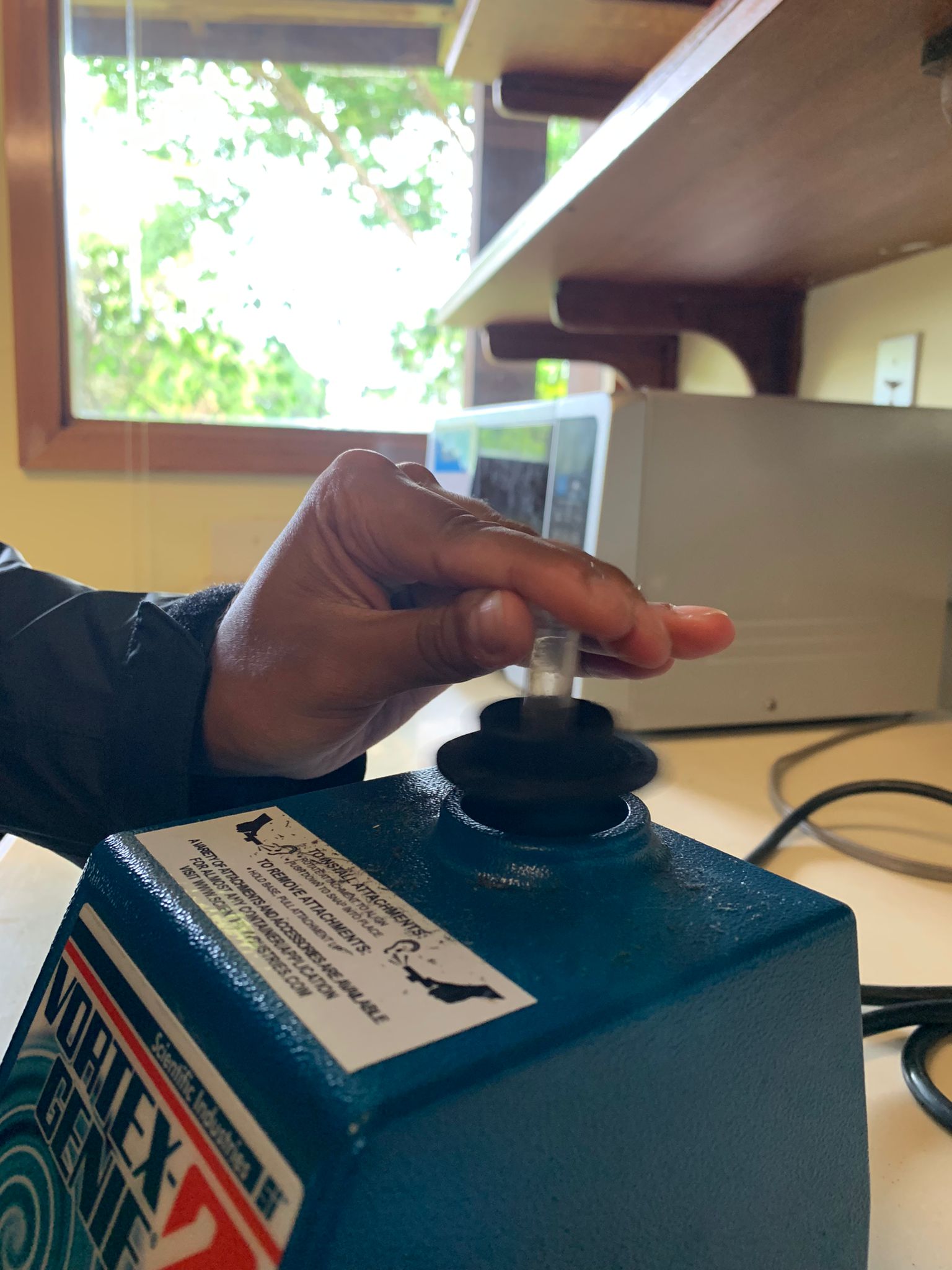
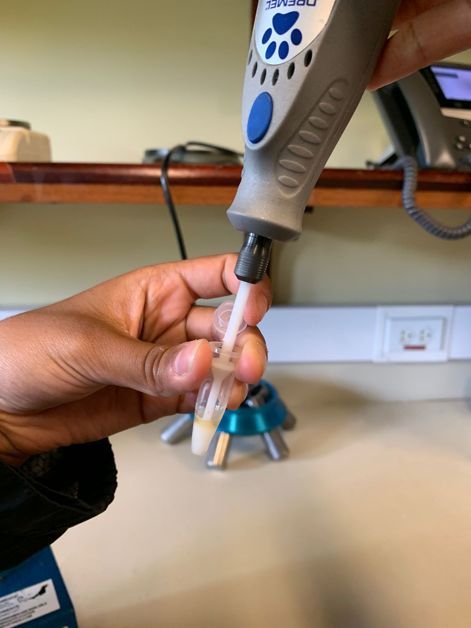
  2. Resuspend pellet using electric homogenizer and/or vortex
  1. Remove a 100 uL aliquot and put into new Eppendorf for dilution
  2. For resuspending use a combination of the vortex and a sewing needle to break up the pellet. Using a syringe and pumping it didn’t go too well.
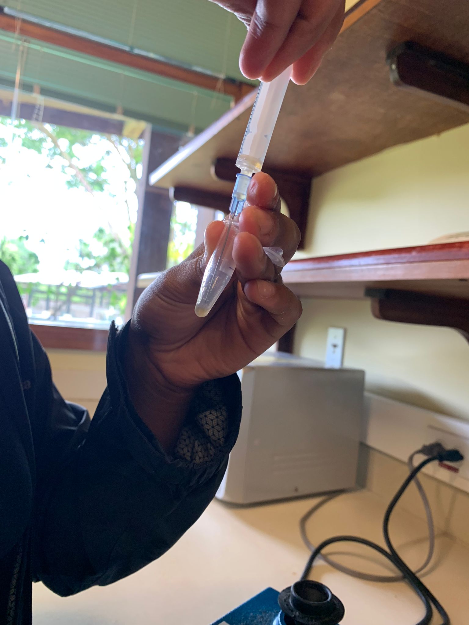
  1. Dilution of the sample will depend on how many zoox there are- start with a 1:1 dilution of the zoox sample and filtered seawater (100 uL homogenate, 100 uL of seawater) ** Try to find a 19-24 gauge hypodermic needle to further separate the zoox cells, draw the sample into and out of the needle multiple times, if you can’t find a needle/syringe skip this step, but there may be clumping

caption: Vortexing zoox count sample with vortex genie.

caption: Resuspending zoox count sample with electric homogenizer.

caption: Drawing sample in and out of hypodermic needle to further separate zoox cells.

  1. Follow the protocol described in the link for counting cells
  2. Dilute the sample as necessary so you are counting between 125-200 cells per “count”. You should have ~25 zoox cells per quadrant (this is for efficiency, so it doesn’t take you forever to count hundreds of cells)
  3. Keep track of the dilution you use- this is necessary for cell calculations

2. Count the zoox

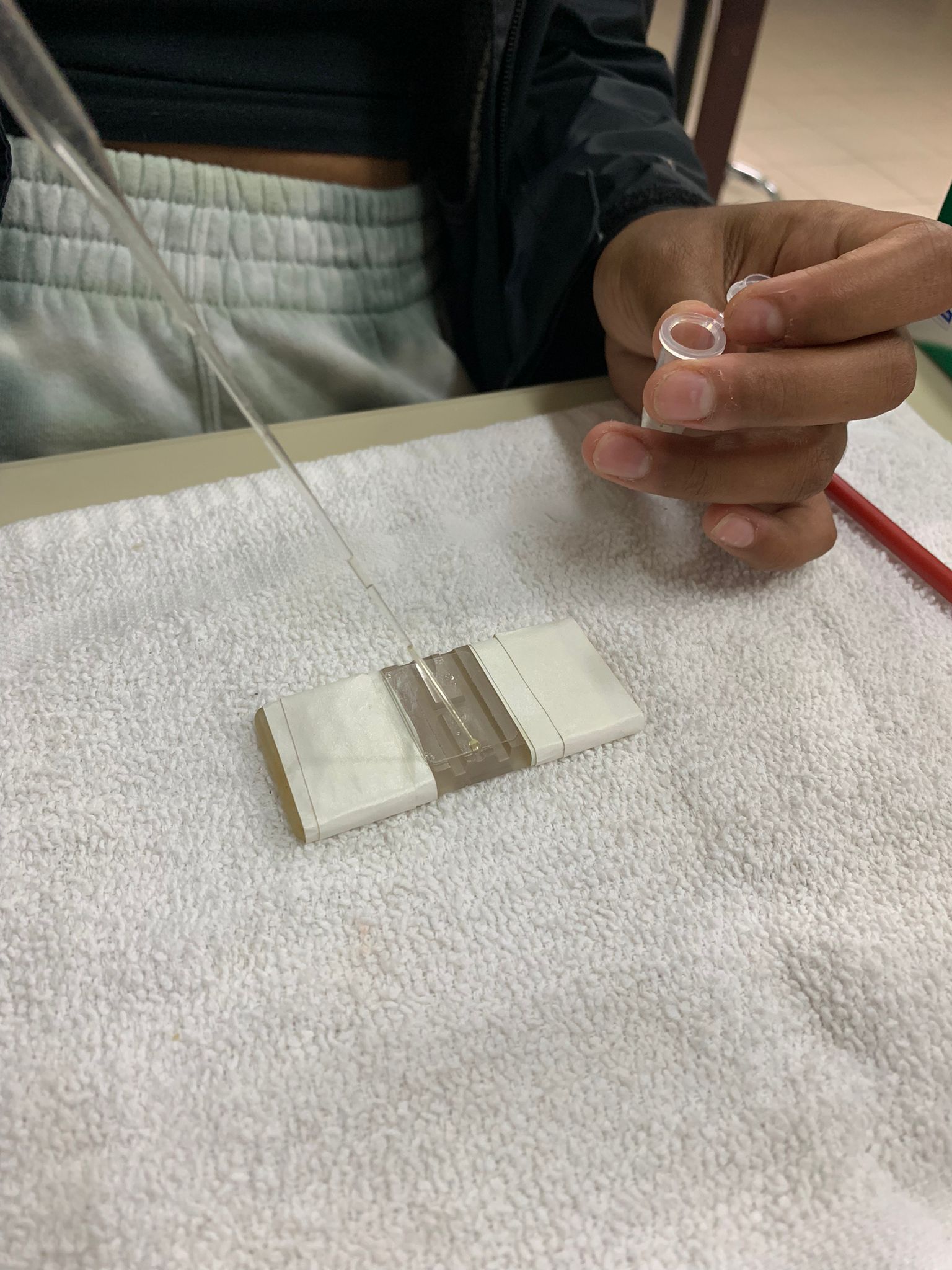
  1. Load the hemocytomter with 10 uL of the diluted sample; Cell Counting With a Hemocytometer: As Easy as 1, 2, 3… To read an overview of counting cells with a hemocytometer. It wouldn’t hurt to look up some of the youtube videos as well.
  2. Do 6 counts per coral fragment- one ‘count’ is the total number of cells counted across the 5 quadrants in one grid (one side of the hemocytometer)- these are quadrants C,D,B,E,F in the image below
  3. The hemocytometer has two grids- so you’ll get two counts per slide. You’ll need to do 3 slides to get the 6 counts per fragment.

caption: Loading hemocytometer with diluted algae sample.

3. Check your numbers

  1. Calculate your cell densities
  2. Look up a couple papers that have zoox counts for respective corals from the region of interest and see that your counts are roughly comparable- this ensures you’re doing the dilution and calculation correctly

title: “PAM Protocol” output: html_document —

Diving PAM II Basic Operation and Protocol

PAM Overview
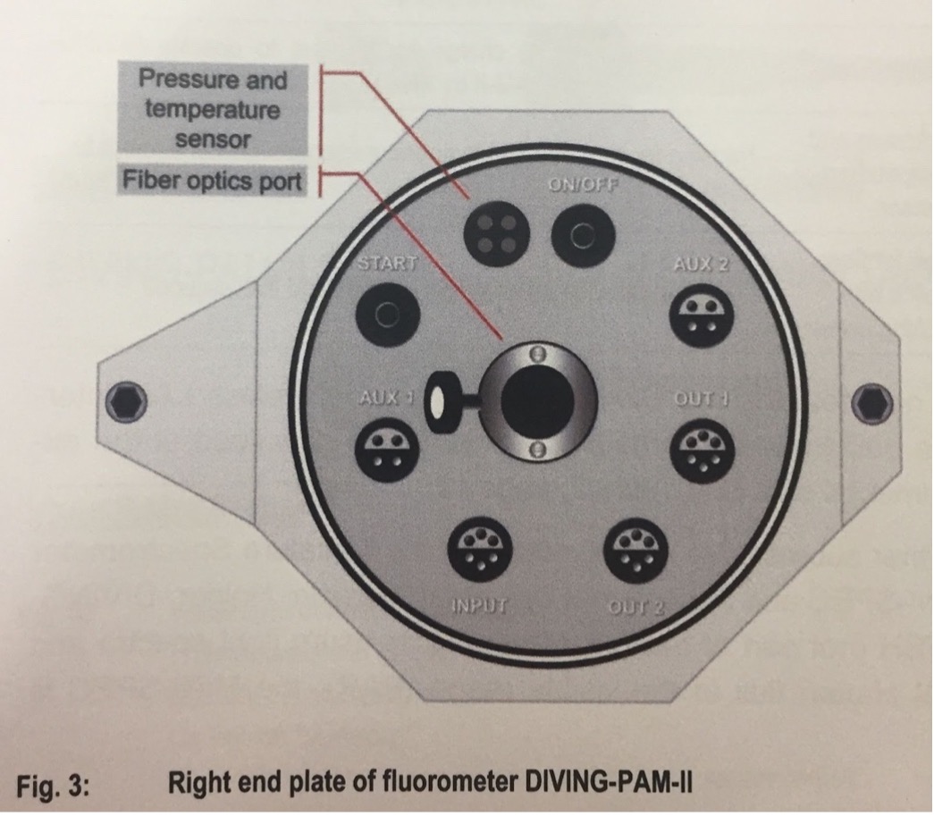
• AUX1/AUX2 connects to Mini Spec or Fiber Optic Oxygen Meter FireSting O2 (← THIS IS AMAZING)

• Fiber Optics Port: Where the fiber optics cable is inserted into the main console.

• INPUT: Interface to charge the battery and to operate the Diving PAM via WinControl-3

• As a note, this protocol as it stands will not cover operating DIVING PAM with WinControl. This protocol is meant to be optimized for in situ measurements

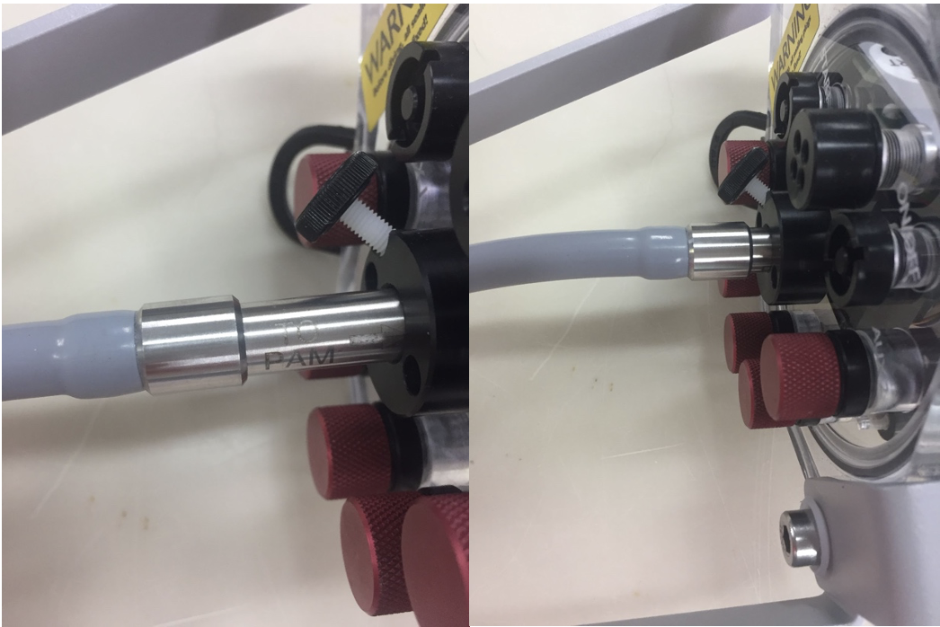
Connecting the Fiber Optic Cord to the PAM: Ensure it is snugly in its port and tighten screw accordingly. There should be no wiggle or play.
Setup for Leafy Material: Seagrasses, Algae, Kelp
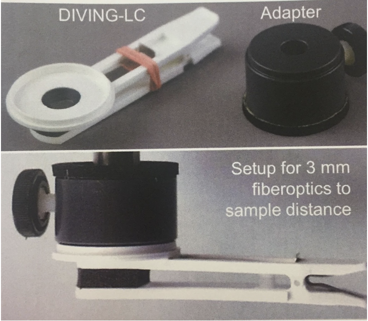
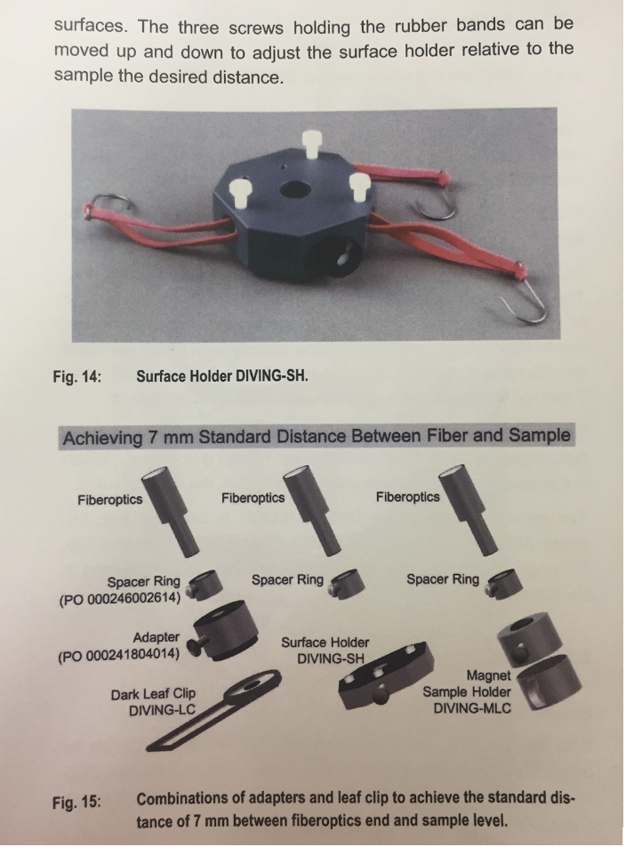
Setup for Coral including diagrams for achieving optimal distance.

Picture4

Picture4

Additional Image of Coral Surface Holder with Dark Adaption
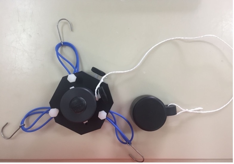
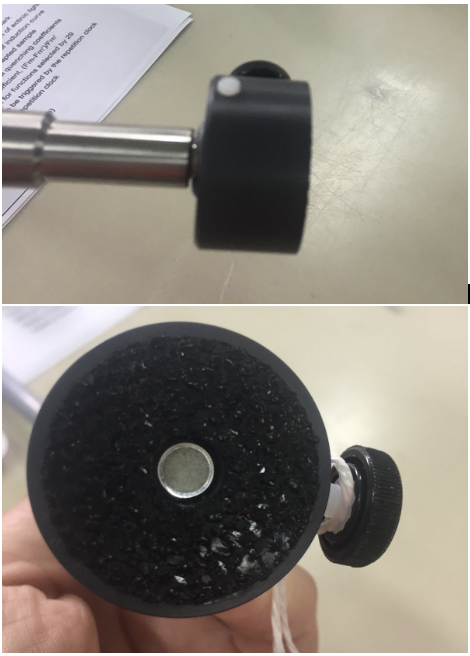
*Note the adaptor is placed directly over the surface holder. There is a slit in the black plug for the fiber optic cord to go through. The black plug attached to the string is buoyant and magnetic. It is meant for ease of use.

Image of fiberoptics inserted into the Adaptor.

Image of fiberoptics inserted into the Adaptor.

Getting the PAM Ready to Rumble

• Unless you are using the MINI-Spec, make sure the PAR is selected for internal PAR sensor. Select Menu ⇒ Sensors ⇒ Use Int. PAR ⇒ On Basic Data Page, select Act.L.

• Adjust GAIN: This is the first of three parameters used to optimize your signal:noise ratio. Noise increases with increasing signal amplification. *Note, Gain should be optimized to your weakest signal (i.e. your most stressed animal).

• Gain is adjusted by referencing your Ft value (i.e. your current fluorescence).

• When adjusting Gain, you want your Ft value to be within range of 300-500.

• To adjust GAIN: Select Menu ⇒ PAM Settings ⇒ Gain ⇒ Select and adjust values between 1-4.

• Adjust DAMPING: Damping suppresses High Frequency Noise. This ranges from 0-20. The higher your damping, the longer your response time.

• Adjusting DAMP vs.GAIN requires play. You will have to optimize this to the values you think are most appropriate for your organism.

• Final range of Ft should be between 300-500. Make sure you record your Gain and Damp. This is oftentimes required to publish. Also, once these values are SET, you cannot change them for the duration of your experiment and data collection period.

• Adjust F-Offset: This determines the background signal for the subtraction from the total signal.

• You MUST F-offset after every change to DAMP and GAIN. You must also adjust F-Offset before EVERY data recording period. This should be done in as close to experimental/field conditions as possible. Ideally, this should be done using experimental treatment or on DIVE in the field.

• Best practice is to ZERO PAM, using a leaf clamp with the metal slider closed.

• Select Menu ⇒ PAM Settings ⇒ Adjust F-Offset.

• It will run for 30s.

• Ft should drop to ~0. Likely between 0-20 with clip on.

make to a table

PAM SETTINGS FOR DIFFERENT CORAL SPECIES SPECIES GAIN DAMPING LIGHT SAT SPACE (mm) Agaricia spp. 2 1 10 7 Acropora cervicornis 1 1 10 7 Diploria labyrinthisformis 3 1 10 7 Siderastrea siderea 1 1 10 7 Porites porites 1 1 10 7 Montastrea cavernosa 2 1 10 7 Orbicella faveolata 1 1 8 7

Taking Measurements Fv/Fm

• Before taking measurements, the organisms should be in its natural experimental condition (light, temp, etc) for a minimum of 24 hours. This is because you want all active photosystems active. Dark Adaptation should last for 20 mins, so the photosystems are most relaxed.

• Select F2. Fv/Fm will show on the main panel.

• Cross validate your values with reported values in the literature.

• Temperature and PAR are the two most important drivers for photosynthesis. In order to make direct comparisons, conditions must be the same or as similar as possible.

Rapid Light Curves

• Again, this requires some play and a defined expectation for outcome. Literature searches are critical to determine the duration of the light curve.

• RLC should start at a PAR value below that of its natural environment. They should be acclimated to experimental conditions and NOT dark adapted.

• If the illumination steps are long enough and refined enough to reach photosynthetic steady state (the asymptote), you can use them as classical light response curves. This means you can calculate alpha, rETRMAX , Ek with considerable confidence.

References

Tunala, Layla Poubel, Frederico T.S. Tâmega, Heitor M. Duarte, and Ricardo Coutinho. 2019. Stress Factors in the Photobiology of the Reef Coral Siderastrea Stellata. Journal of Experimental Marine Biology and Ecology. 519: 151188. https://doi.org/10.1016/j.jembe.2019.151188.

Manzello, D., M. Warner, E. Stabenau, J. Hendee, M. Lesser, and M. Jankulak. 2009. Remote Monitoring of Chlorophyll Fluorescence in Two Reef Corals during the 2005 Bleaching Event at Lee Stocking Island, Bahamas. Coral Reefs 28 (1): 209–14. https://doi.org/10.1007/s00338-008-0455-7.

Cunning, Ross, Rachel N. Silverstein, and Andrew C. Baker. 2018. Symbiont Shuffling Linked to Differential Photochemical Dynamics of Symbiodinium in Three Caribbean Reef Corals. Coral Reefs 37 (1): 145–52. https://doi.org/10.1007/s00338-017-1640-3.

Finelli, C. M., B. S. Helmuth, N. D. Pentcheff, and D. S. Wethey. 2007. Intracolony Variability in Photosynthesis by Corals Is Affected by Water Flow: Role of Oxygen Flux. Marine Ecology Progress Series 349: 103–10. https://doi.org/10.3354/meps07101.
title: “MIG Bleaching Analysis Protocol” output: html_document —

Mean Intensity Grey (MIG) Bleaching Analysis

• Coral bleaching is a visually notable phenomenon where physiological stress results in loss of the coral host’s pigmented endosymbiotic algae, known as Symbiodinium or zooxanthellae. This leaves the coral animal’s tissues white or “bleached” in color. Through photography and digital image analysis of corals in- or ex-situ, Mean Intensity Grey (MIG), or percent whiteness, has been shown to be highly correlated with zooxanthellae and chl-a densities (Chow et al., 2016, Amid et al., 2018) and can give robust estimates of bleaching intensity.

This method is a simple and non-destructive tool that removes observer bias and provides a more precise, continuous value for coral bleaching intensity as opposed to categorical chart data such as that obtained using references such as the Coral Health Chart (Siebeck et al., 2006).

PICTURE SET-UP

Submerge coral fragments and ruler with white standard in shallow bin under camera on stand. Set camera to manual mode (M) and turn on flash so no shadows appear on surface of corals. Take photo and see where narrow flash appears on image and arrange corals so this does not appear over them.

Organize fragments so individual numbers, white standard and treatment tag are visible.

IMAGE ANALYSIS

• Name each photo according to tank number and oxygen treatment, ex. ppor_T1_N, and put in folder with species and temp treatment.

• Open ImageJ and select File -> Open, and select photo to be analyzed.

• Select Image -> Type -> 8-bit, this will convert image to greyscale.

• Select oval from ImageJ toolbar and draw a circle over a fragment and select Analyze -> set measurements… and check only mean grey value -> Ok

• Using the circle selection tool, draw a small circle approximately 1 cm below growing tip for P. porites across the width of the fragment, making sure to only include living tissue. Hit control-m to return MIG measurements. Draw a circle on the white background without specs and glare or shadows and take measurement, this will be used as the reference MIG value to normalize fragment colorimetric values.

For porites and acropora, circle was drawn approximately 1 cm below the growing tip from the same area that was sampled for zooxanthellae density counts.

References

Amid, C., Olstedt, M., Gunnarsson, J.S. et al. Additive effects of the herbicide glyphosate and elevated temperature on the branched coral Acropora formosa in Nha Trang, Vietnam. Environ Sci Pollut Res 25, 13360–13372 (2018). https://doi.org/10.1007/s11356-016-8320-7

Chow MH, Tsang RHL, Lam EKY, Ang P. 2016. Quantifying the degree of coral bleaching using digital photographic technique. Journal of Experimental Marine Biology and Ecology.

Siebeck, U.E., Marshall, N.J., Kluter, A., Hoegh-Guldberg, O., 2006. Monitoring coral bleaching using a colour reference card. Coral Reefs 25, 453–460.